Governing equations
In order to arrive at a solution for stress equilibrium and strain compatibility the solver of the mechanical boundary value problem needs to know the stress response of the integration points to a given deformation. More precisely, the solver requests a stress that results from a change in the local deformation gradient from $\tnsr F(t_0)$ at the beginning $t_0$ of the increment to $\tnsr F(t)$ at the end $t$ of the increment, with $\Delta t = t - t_0$ being the time step. The type of stress measure that is required depends on the solver and might be a Cauchy stress $\tnsr \sigma$ or a first Piola–Kichhoff stress $\tnsr P$. Both measures can, however, be calculated from any other stress measure by simple transformation rules. Here, the connection between stress and strain is based on the second Piola–Kirchhoff stress $\tnsr S$ as a function of the elastic deformation gradient $\tnsr F_\text e$ in terms of an elastic constitutive law. \begin{equation} \label{eq:constitutive S} \tnsr S = \tnsr S(\tnsr F_\text e) \end{equation}Hence, in order to calculate the stress response of the integration point, one has to know the elastic deformation gradient at the end of the increment $\tnsr F_\text e(t)$. In contrast to the total deformation gradient, this is, however, not known a priori. It depends on the partitioning of the deformation gradient into elastic and plastic part. \begin{equation} \label{eq:constitutive Fe} \tnsr F_\text e = \tnsr F {\tnsr F_\text p}^{-1} \end{equation} While the material initially deforms purely elastic, the proportion of the plastic deformation will increase once the yield point of the material is reached.
The rate with which the plastic deformation gradient $\tnsr F_\text p$ evolves is determined by the plastic velocity gradient $\tnsr L_\text p$ by means of a nonlinear ordinary differential equation. \begin{equation} \label{eq:constitutive Fp} \dot{\tnsr F}_\text p = \tnsr L_\text p \tnsr F_\text p \end{equation}
The plastic velocity gradient describes the speed of the permanent deformation of a material and is part of the plastic constitutive behavior. It depends on the second Piola–Kirchhoff stress acting as a driving force, as well as on the microstructure of the material represented by some state variables $\vctr \omega$. \begin{equation} \label{eq:constitutive Lp} \tnsr L_\text p = \tnsr L_\text p(\tnsr S , \vctr\omega) \end{equation} The microstructure at the material point evolves simultaneously with the kinematic quantities. So, additionally, there is a second constitutive equation that describes the evolution rate of the state variables. \begin{equation} \label{eq:constitutive dotstate} \dot{\vctr\omega} = \dot{\vctr\omega}(\tnsr S , \vctr\omega) \end{equation} In some cases it might be necessary to express the change in the microstructure in terms of an instantaneous jump rather than by a rate of change. For this case, a third constitutive equation that is not formulated as rate equation can equally be defined. \begin{equation} \label{eq:constitutive deltastate} \Delta{\vctr\omega} = \Delta{\vctr\omega}(\tnsr S , \vctr\omega) \end{equation}Equations \eqref{eq:constitutive S} to \eqref{eq:constitutive deltastate} govern the evolution of stress, strain, and microstructure and have to be solved at the level of each material point. Due to the nonlinear coupling of the unknown variables, this is not easily possible. In order to reduce the complexity of the problem, we decouple the evolution of the microstructure (i.e. state variables) from the evolution of the other variables. This can be reasoned by the fact that the microstructure usually evolves slower than stress and strain (akin to a Born–Oppenheimer approximation). Then, the set of equations can be solved in two levels:
- In an inner level, the stress $\tnsr S$ is obtained by solving equations \eqref{eq:constitutive S} to \eqref{eq:constitutive Lp} at constant state $\vctr\omega$.
- In an outer level, the state $\vctr\omega$ is obtained by solving equations \eqref{eq:constitutive dotstate} and \eqref{eq:constitutive deltastate} for a given stress $\tnsr S$.
Inner level of stress integration
Linearized Backward Euler
In order to solve the set of equations \eqref{eq:constitutive S} to \eqref{eq:constitutive Lp}, we approximate the time derivative in \eqref{eq:constitutive Fp} by a backward finite difference, and we obtain an implicit equation for the plastic deformation gradient at the end of the increment. \begin{equation*} \frac{\tnsr F_\text p(t) - \tnsr F_\text p(t_0)}{\Delta t} = \tnsr L_\text p(t) \tnsr F_\text p(t) \end{equation*} This equation can be solved for $\tnsr F_\text p(t)$ by simple linear algebra. \begin{equation*} \tnsr F_\text p(t) = {\left(\tnsr I - \Delta t\; \tnsr L_\text p(t)\right)}^{-1} \tnsr F_\text p(t_0) \end{equation*} Inserting this into equation \eqref{eq:constitutive Fe} one obtains an equation for the elastic deformation gradient at the end of the increment. \begin{equation*} \tnsr F_\text e(t) = \tnsr F(t) \; {\tnsr F_\text p}^{-1}(t_0) \left(\tnsr I - \Delta t\; \tnsr L_\text p(t)\right) \end{equation*} By this linearization procedure, one obtains a system of three algebraic equations with three unknowns $\tnsr S(t)$, $\tnsr F_\text e (t)$, and $\tnsr L_\text p (t)$: \begin{align} \tnsr S (t) &= \tnsr S(\tnsr F_\text e (t)) \nonumber \\ \tnsr F_\text e(t) &= \tnsr A \left(\tnsr I - \Delta t\; \tnsr L_\text p(t)\right) \label{eq:backwardSystem} \\ \tnsr L_\text p (t) &= \tnsr L_\text p(\tnsr S (t))\nonumber \end{align} where the known quantity $\tnsr F(t) \; {\tnsr F_\text p}^{-1}(t_0)$ is substituted by $\tnsr A$ for brevity and corresponds to a fully elastic predictor.
For later use, the derivative of the elastic deformation gradient with respect to the plastic velocity gradient follows as \begin{align} \label{eq:backwardFeDerivative} \tnsr F_\text e,_{\scriptscriptstyle\tnsr L_\text p} &= \left[\tnsr A \left(\tnsr I-\Delta t \; \tnsr L_\text p\right)\right],_{\scriptscriptstyle\tnsr L_\text p} = -\Delta t \, \tnsr A \tnsrfour I = -\Delta t \, \tnsr A \otimes\tnsr I \end{align} It is useful to rewrite this in index notation: \begin{align*} \frac{\partial {F_\text e}_{\,ij}}{\partial {L_\text p}_{\,kl}} \vctr g^i \otimes \vctr g_k \otimes \vctr g_l \otimes \vctr g^j &= -\Delta t \, A_{i\cdot}^{\phantom i k} \delta^l_j \,\vctr g^i \otimes \vctr g_k \otimes \vctr g_l \otimes \vctr g^j \end{align*}
Exponential Forward Euler
An alternative way to solve the set of equations \eqref{eq:constitutive S} to \eqref{eq:constitutive Lp} is by considering the correct solution \begin{equation*} \tnsr F_\text p(t) = \exp\left(\Delta t\,\tnsr L_\text p(t)\right) \tnsr F_\text p(t_0) \end{equation*}
Inserting this into equation \eqref{eq:constitutive Fe} one obtains an equation for the elastic deformation gradient at the end of the increment. \begin{align*} \tnsr F_\text e(t) &= \tnsr F(t) \; {\tnsr F_\text p}^{-1}(t_0) \exp\left(- \Delta t\; \tnsr L_\text p(t)\right) \\ &= \tnsr F(t) \; {\tnsr F_\text p}^{-1}(t_0) \left( \tnsr I -\Delta t \;\tnsr L_\text p(t) + \frac{\Delta t^2}{2!}{\tnsr L_\text p}^2 (t) + \mathcal O(\Delta t^3)\right) \end{align*} By truncating the series expansion after second order, one obtains a system of three algebraic equations with three unknowns $\tnsr S(t)$, $\tnsr F_\text e (t)$, and $\tnsr L_\text p (t)$: \begin{align} \tnsr S (t) &= \tnsr S(\tnsr F_\text e (t)) \nonumber \\ \tnsr F_\text e(t) &= \tnsr A \left( \tnsr I -\Delta t \;\tnsr L_\text p(t) + \frac{\Delta t^2}{2!}\tnsr L_\text p(t) \right) \label{eq:exponentialSystem} \\ \tnsr L_\text p (t) &= \tnsr L_\text p(\tnsr S (t))\nonumber \end{align} where the known quantity $\tnsr F(t) \; {\tnsr F_\text p}^{-1}(t_0)$ is substituted by $\tnsr A$ for brevity and corresponds to a fully elastic predictor.
For later use, the derivative of the elastic deformation gradient with respect to the plastic velocity gradient follows as \begin{align} \label{eq:exponentialFeDerivative} \tnsr F_\text e,_{\scriptscriptstyle\tnsr L_\text p} &= \left[\tnsr A \exp\left(- \Delta t\; \tnsr L_\text p \right)\right],_{\scriptscriptstyle\tnsr L_\text p}\nonumber \\ &= \tnsr A \left[ -\Delta t \tnsr I \otimes \tnsr I + \frac{\Delta t^2}{2!}\left( \tnsr L_\text p \otimes \tnsr I + \tnsr I \otimes \tnsr L_\text p \right) \right]\nonumber \\ &= -\Delta t \, \tnsr A \otimes\tnsr I + \frac{\Delta t^2}{2}\left( \tnsr A \tnsr L_\text p \otimes \tnsr I + \tnsr A \otimes \tnsr L_\text p\right)\;. \end{align} It is useful to rewrite this in index notation: \begin{align*} \frac{\partial {F_\text e}_{\,ij}}{\partial {L_\text p}_{\,kl}} \vctr g^i \otimes \vctr g_k \otimes \vctr g_l \otimes \vctr g^j &= -\Delta t \, A_{i\cdot}^{\phantom i k} \delta^l_j \\ &\phantom = +\frac{\Delta t^2}{2} \left( A_{i m} {L_\text p}^{m k} \delta^l_j + A_{i\cdot}^{\phantom i k} {L_\text p}^{l}_j \right) \vctr g^i \otimes \vctr g_k \otimes \vctr g_l \otimes \vctr g^j \end{align*}
Consistent solution
The systems \eqref{eq:backwardSystem} and \eqref{eq:exponentialSystem} can be solved by a Newton–Raphson scheme by either minimizing the residuum in $\tnsr S$, $\tnsr F_\text e$, or $\tnsr L_\text p$. Choosing the norm of the residuum in $\tnsr S$ as an objective function has the advantage that the inverse that is needed for the Newton–Raphson procedure is only $6\times6$ compared to $9\times9$ for $\tnsr L_\text p$ or $\tnsr F_\text e$, since the stress tensor is symmetric, while $\tnsr L_\text p$ and $\tnsr F_\text e$ are not. However, it is much harder to guess and correct for $\tnsr S$ than for $\tnsr L_\text p$, since the plastic velocity is usually very sensitive to a change in the stress. For this reason the Newton–Raphson scheme is chosen around $\tnsr L_\text p$ with the advantage of fast convergence at the expense of a higher cost per iteration step.
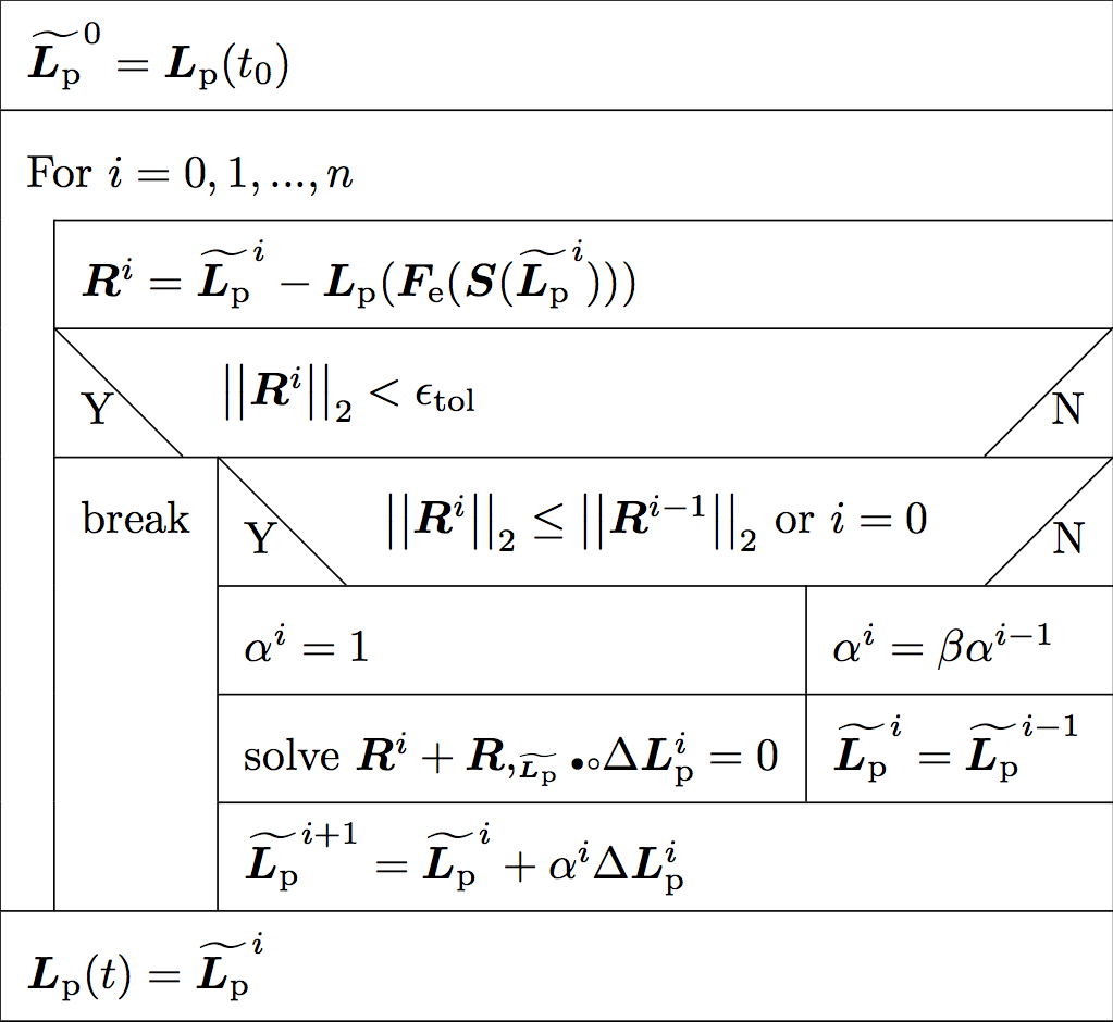
The residuum in $\tnsr L_\text p$ for the $i$th iteration is defined as \begin{align} \label{eq:residuum} \tnsr R^i = {\widetilde{\tnsr L_\text p}}^i - \tnsr L_\text p (\tnsr S(\tnsr F_\text e ({\widetilde{\tnsr L_\text p}}^i))) \end{align} and the objective function, which will be minimized, as the Frobenius norm of the residuum: \begin{align} \min_{\tnsr L_\text p} \|\tnsr R\|_2 \qquad\text{with}\qquad \|\tnsr R\|_2 = \sqrt{\tnsr R : \tnsr R} \end{align} The minimization procedure employs a modified Newton–Raphson scheme with variable step length $\alpha$ (see figure 1). The correction of the $i$th guess for $\tnsr L_\text p$ is based on the derivative of the residuum and is obtained by solving the following linear equation for $\Delta\tnsr L_\text p^i$ (cf. tensor notation scheme). \begin{align} \label{eq:Lp correction} \tnsr R^i + \tnsr R,_{\scriptscriptstyle\widetilde{\tnsr L_\text p}} \; \dblContInOut \; \Delta\tnsr L_\text p^i &= 0 \end{align} This equation can be solved by means of any method for linear equation systems. The resulting correction $\Delta\tnsr L_\text p$ is used to update the guess for $\tnsr L_\text p$. The updated guess is only accepted if the residuum is decreased in the next step. Otherwise, subsequent guesses are based on the same (old) jacobian, but with a step that is cutbacked by a factor $\beta$ (usually chosen equal to $0.5$) until the solution has improved. This procedure ensures faster convergence both from the viewpoint of iterations and computational effort, because the costly solution to equation \eqref{eq:Lp correction} is not needed in every iteration. The Newton–Raphson scheme is regarded converged when the norm of the residuum drops below a given tolerance $\epsilon_\text{tol}$. The derivative of the residuum that is needed in equation \eqref{eq:Lp correction} follows from equation \eqref{eq:residuum} as \begin{align} \label{eq:residuum derivative} \tnsr R,_{\scriptscriptstyle\widetilde{\tnsr L_\text p}} &= \tnsrfour I - \tnsr L_\text p,_{\scriptscriptstyle\tnsr S} \; \dblContInOut \; \tnsr S,_{\scriptscriptstyle\tnsr F_\text e} \; \dblContInOut \; \tnsr F_\text e,_{\scriptscriptstyle\widetilde{\tnsr L_\text p}} \end{align} From the three derivatives in the product at the end of this equation only the last one is independent of the material's constitutive behavior. The other two derivatives in the product of equation \eqref{eq:residuum derivative} dependent on the plastic (${\tnsr L_\text p},{\scriptscriptstyle\tnsr S}$) and elastic ($\tnsr S,{\scriptscriptstyle\tnsr F_\text e}$) constitutive law.Outer level of state integration
Fixed-point iteration scheme
Explicit Euler integrator
Adaptive Euler integrator
Fourth-order explicit Runge-Kutta integrator
Fifth-order adaptive Runge-Kutta integrator


| I | Attachment | Action | Size | Date | Who | Comment |
|---|---|---|---|---|---|---|
| |
NewtonRaphson.pdf | manage | 95 K | 17 Jan 2014 - 08:10 | ChristophKords | |
| |
NewtonRaphson.png | manage | 67 K | 20 Oct 2014 - 21:30 | PhilipEisenlohr | Newton--Raphson Scheme |
Topic revision: 31 Jan 2015, PhilipEisenlohr
Ideas, requests, problems regarding DAMASK? Send feedback
§ Imprint § Data Protection